NCA-Flow for Ultrasound
Three obstacles, one root cause
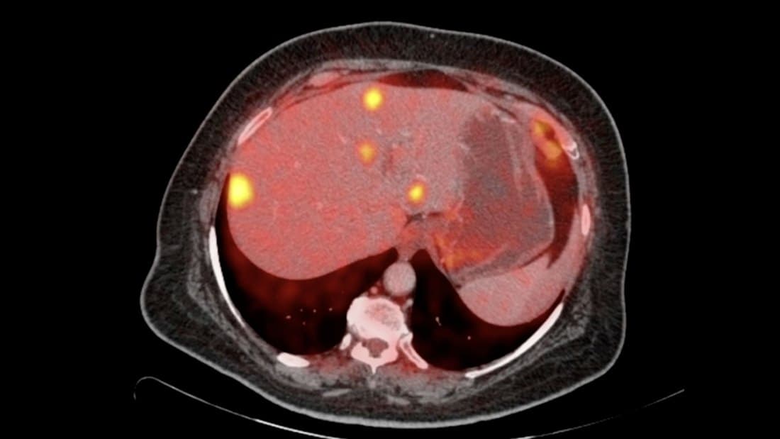
An ultrasound-guided biopsy. The tissue will not hold still — it deforms under the probe and moves with breathing, so the target is not where the earlier scan said it was. The operator has a moving 2D slice and what they feel through the needle, and that feel fades once the tool gets long or a robot is holding it. One thing underlies everything that could help: from a pair of frames, how did the tissue move, at every pixel.
Physics mismatch
Optical flow assumes brightness constancy. Speckle is an interference pattern — under deformation it changes rather than translating.
Temporal design flaw
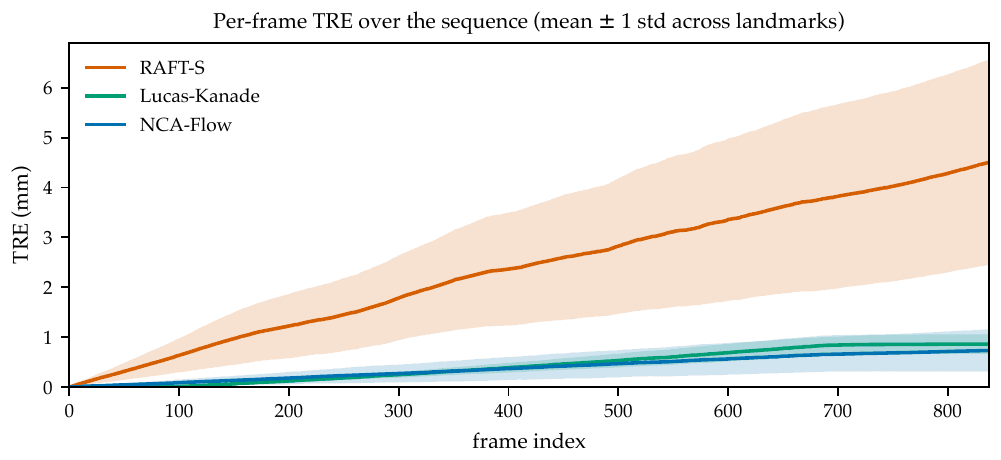
Per-frame re-detection injects jitter. Displacement is accumulated, and differentiating into strain amplifies it. 0.31 mm a frame is small until you stack 800.
Parameter bloat
10⁵–10⁸ trainable parameters in every learned baseline — latency and memory that point-of-care ultrasound cannot afford.
All three follow from one fact: a pixel's displacement is set almost entirely by its immediate neighbourhood — there is no distant structure to recognise. Ultrasound displacement is a fundamentally local problem — which is exactly what a neural cellular automaton is built around. Classification, segmentation and static registration had all been done with automata. Frame-to-frame motion in ultrasound had not.
One small rule, applied everywhere, iterated
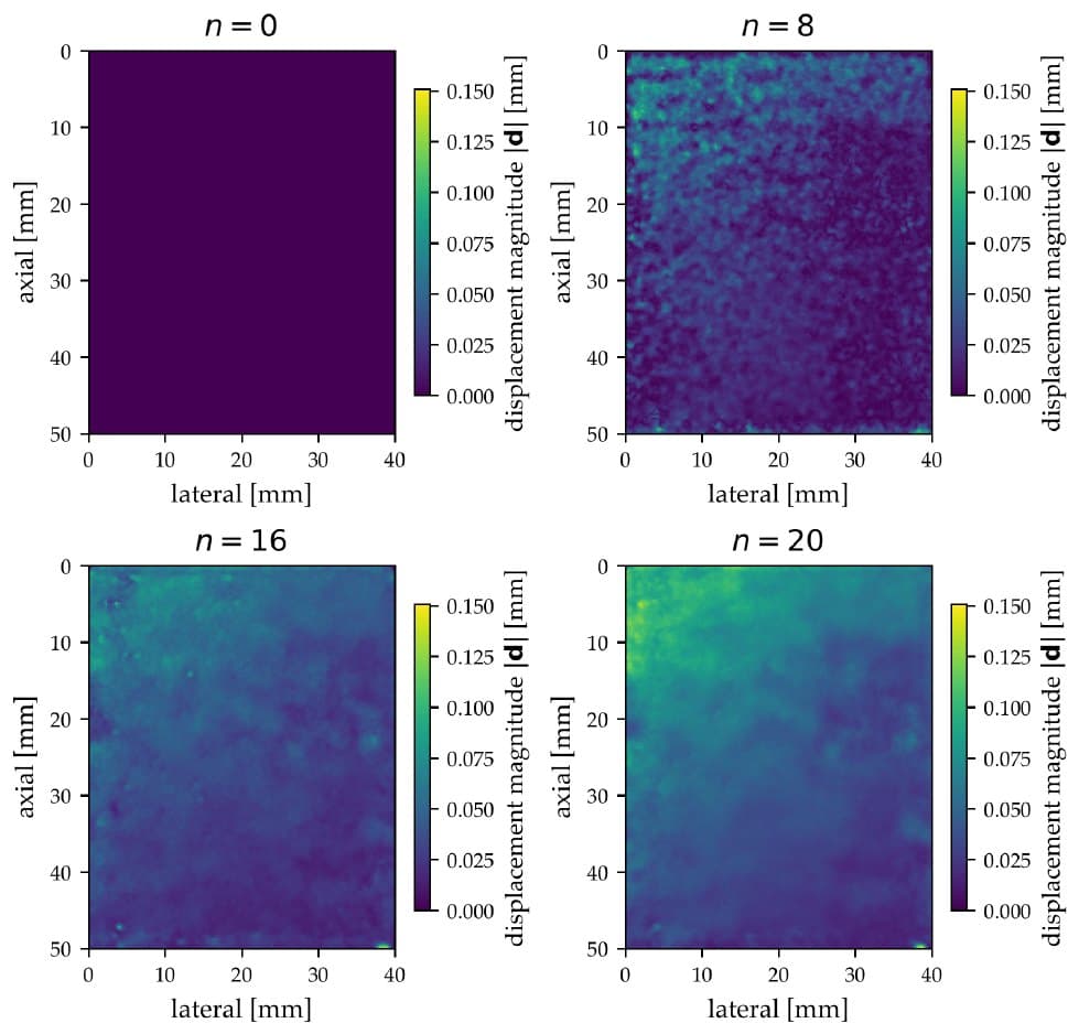
Each pixel holds 12 channels: two displacement, eight hidden, and the two frames as read-only context. All zero at the start, so the field grows from nothing.
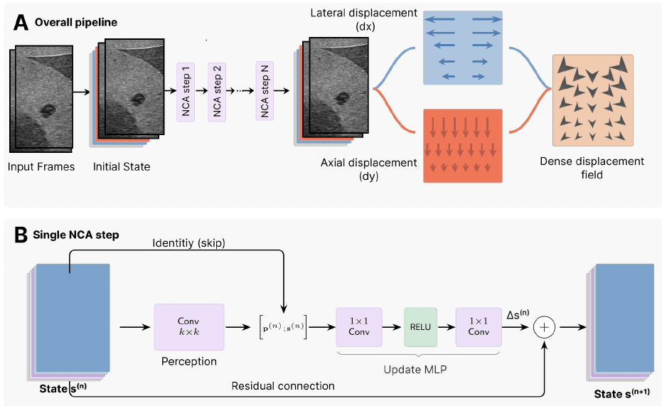
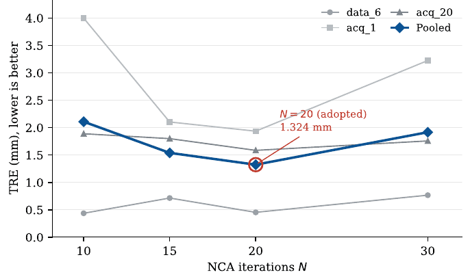
The form is additive — refine, don't replace. Iterated to N = 20 the receptive field reaches ≈41×41 px, which spans the scale the motion is coherent over. Because the rule is shared across every pixel and every step, the 16,714 parameters do not grow with image size.
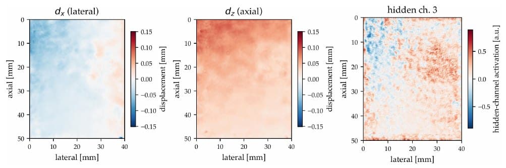
More freedom, worse result
How should a cell read its neighbourhood — a learned convolution, a fixed bank of classical differential filters, or a hybrid?
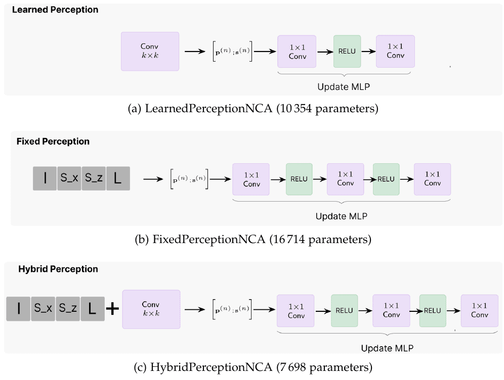
The fixed set wins: identity, the two Sobel gradients and the Laplacian, none of them trained — the same operators classical motion estimation is built on. Learning them instead is 1.8× worse; the hybrid 1.35×. And the hybrid contains the fixed set as a special case — switch off its learned half and you get it back exactly — yet it still trained to a worse result at every size tried. So perception is free, and all 16,714 parameters sit in the update network.
Kernel size points the same way and is decisive: k = 3 is nearly an order of magnitude better than k = 7. A wider reach per step buys slightly better single-frame predictions, then accumulates hundreds of unrolled steps of drift. Small kernels are not marginally better here — they are necessary.
Train where truth exists, adapt where it doesn't
Dense ground truth for real ultrasound cannot be observed at all — so pre-training happens in simulation and adaptation happens on sparse landmarks.
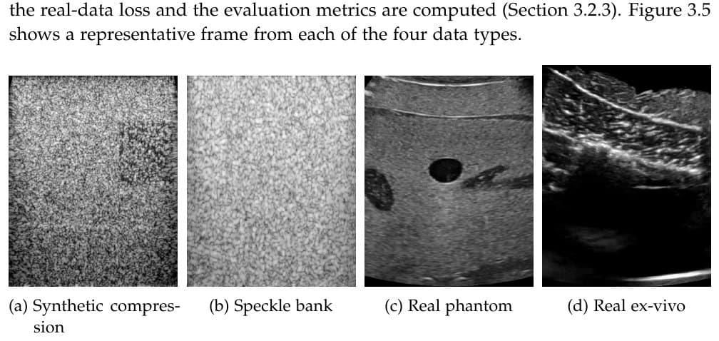
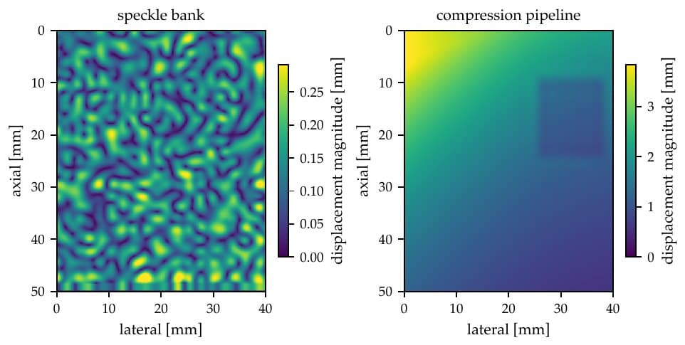
Fine-tuning predicts the dense field, reads it off at the landmarks, and regresses. That roughly halves the pooled error, 1.444 → 0.674 mm. A stream of synthetic pairs stays in the loss so the model does not bend itself to a few hundred points — and to be precise about what that anchor does: it buys retention, not accuracy. Dropping it leaves the pooled mean nominally lower (0.651), well inside the noise, but the un-anchored variant degrades 2.91× on the speckle family it stops seeing. It costs nothing measurable and preserves behaviour, so it stays on that basis.
How it's judged
- Metrics
- TRE — how far off the landmarks end up, in mm. MTE — the same at every annotated frame, which catches a model that wanders mid-sequence and lands near the right place by luck. LNCC — how steady the strain pattern is over time. Folding — whether the deformation is physically possible at all.
- Data
- Three clips with no subject shared between them, and 976 landmarks. Two ex-vivo tissue, one phantom.
- Baselines
- Learned: StrainNet-f, StrainNet-l, DICTr, RAFT-S. Classical: Lucas-Kanade, Farnebäck.
Not a fair fight: Lucas-Kanade is an upper reference, not an independent win — the ground-truth landmarks were propagated by a tracker of its own family. Pooled, the two tie: NCA-Flow takes the lower endpoint error and folds far less, Lucas-Kanade the lower trajectory error (0.325 against 0.346). The learned baselines carry no such dependency.
LNCC is reported, not leaned on. Every method lands between 0.97 and 0.99, so it saturates and does not discriminate. The comparison rests on TRE, MTE and folding.
Accuracy without scale
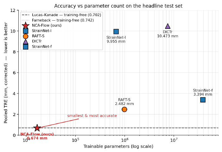
More accurate than every learned baseline, at between 40× and 2,314× fewer parameters — and the margin does not come from fine-tuning.
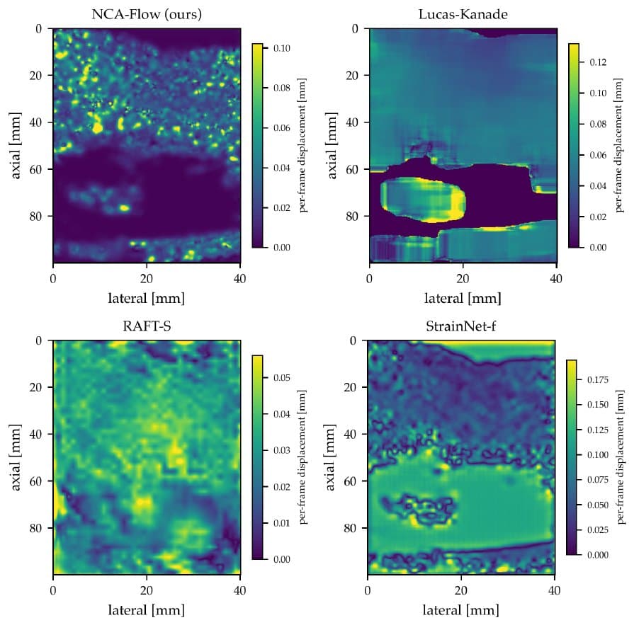
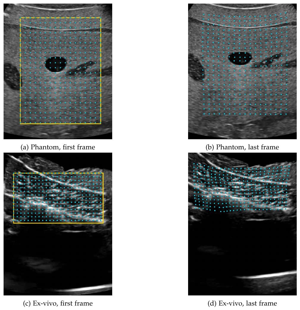
How to read it: look for lines crossing. A crossed cell is tissue mapped through itself — which cannot physically happen under compression.
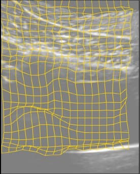
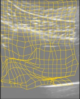
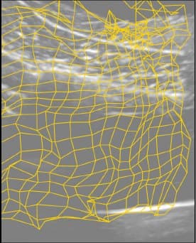
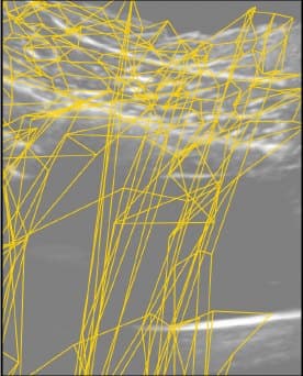
Stays close to regular. Neighbouring pixels agree about where they are going.
4.55% pooled over all three clips · 7.5% on this frame, the worst of the ex-vivo clip.
Folding does not imply a discontinuous gradient — a smooth contraction strong enough to invert the map folds everywhere. The criterion is the sign of det(I + ∇u).
What this does not establish
Whether it helps in the clinic is still an open question.
- Non-clinical. No in-vivo data, no pathology, no operator or machine variation.
- Ground truth. Reference landmarks are Lucas-Kanade derived, so not independent of one baseline.
- 2D only. A single plane; blind to out-of-plane motion.
- Synthetic realism. The simulator was configured by eye, not against a measured criterion.
- B-mode ceiling. Log compression discards the phase correlation estimators exploit.
- The open claim. Tracking decorrelating speckle is consistent with the locality argument — not a test of it.
- In-vivo validation. Past controlled tissue, to live tissue and real variation.
- Less annotation. Self-supervised adaptation would remove the Lucas-Kanade dependence — the change that would do most.
- Temporal NCA. Carry state across frames instead of solving each pair alone.
- RF / phase input. The one change that lifts the B-mode ceiling rather than working beneath it.
- Volumetric. Extend the local rule to a 3D grid.
- Publication. Submitted to MICCAI 2026, not accepted. Most of the above is what would strengthen it.
The three obstacles, answered
Inductive bias over scale.
Tracks decorrelating speckle
0.674 mm on real ex-vivo and phantom tissue, where the larger learned methods degrade.
Drift stays flat
0.09 mm per 100 frames, ending 838 frames at 0.74 mm. RAFT-S ends at 4.53.
Accuracy without scale
16,714 parameters, more accurate than StrainNet-f at 2,314× the size.
To our knowledge, the first neural cellular automaton for pairwise dense motion estimation in B-mode ultrasound. What stays open is why — that locality is the reason this works is consistent with these results, not established by them.