Bachelor Thesis:CarToGraph

Autonomous vehicles need near-perfect object detection to ensure safety. But current algorithms treat each car detection independently, completely ignoring that real-world objects follow spatial patterns.

Cars in parking lots form grids. Highway traffic flows in lanes. Pedestrians cluster at crosswalks.

The critical gap: Existing systems ask 'Is this a car?' instead of 'Is this a car AND does it fit the spatial pattern of surrounding cars?'

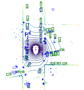
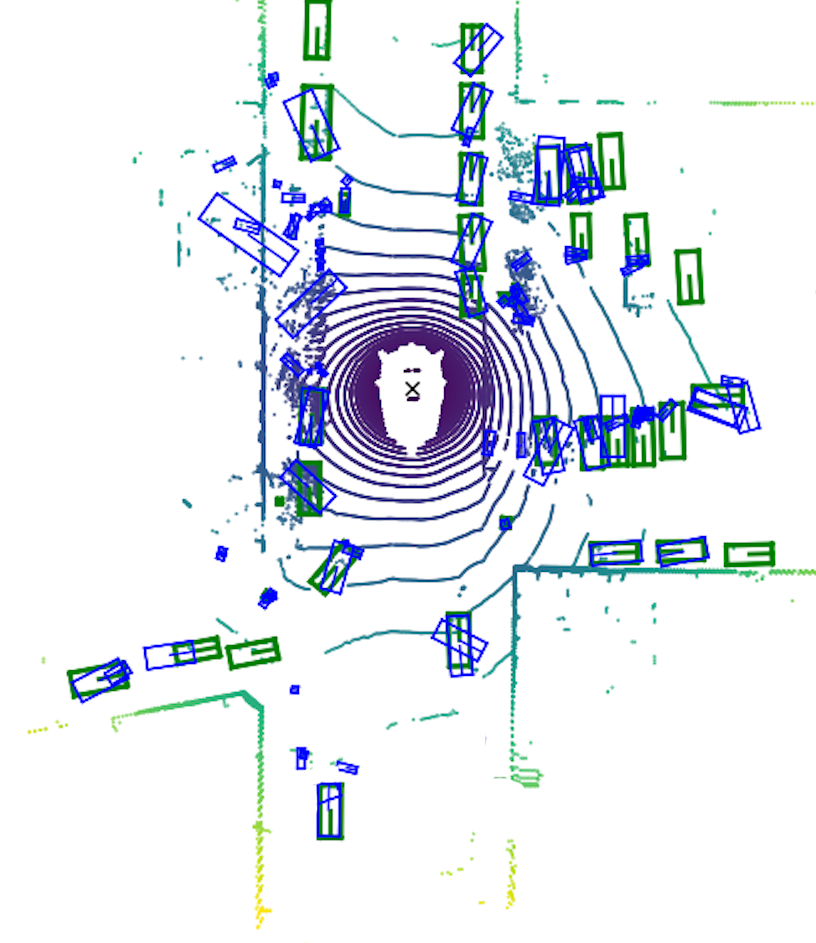
We transform car detections into mathematical graphs. Each car becomes a node. Spatial relationships become edges. Now we can compare predicted patterns against reality using graph theory.

Instead of asking 'Is this a car?' we ask 'Does this car fit the spatial pattern?'

The system analyzes connectivity patterns to validate detections. Cars in parking lots should form grid-like connections. Highway traffic should flow in lane formations. Any detection that breaks these patterns gets flagged.

I experimented with three graph generation methods to capture different spatial relationships:

MST (Minimum Spanning Tree): Creates the simplest possible connected graph. Clean and efficient, but sometimes too sparse.

KNN (K-Nearest Neighbors): Each car connects to its k closest neighbors. Rich local detail, gave me a consistent 2.3% improvement.

Double MST: My breakthrough - applying MST twice with different criteria. Balances global connectivity with local richness. This gave me the best results at 4.1%.

The key insight: different scenes need different connectivity patterns, but the right graph structure can capture them all.

I designed three complementary loss functions to capture what makes a spatially correct detection:

Connectivity Loss: Counts how many neighbors each car has. If predicted has 2 connections but ground truth has 4, we penalize the difference. Simple counting, powerful for finding local errors.

Triangle Loss: Counts three-way connections between cars. More triangles indicate tighter clustering. A missing car breaks multiple triangles at once - that's how we catch it.

Laplacian Loss: Compares the eigenvalues of the graph Laplacian matrices - essentially the graph's "fingerprint". This captures global structure without needing to match individual cars.

The beauty of this approach: you don't need to start over.

After testing different strategies, I found the sweet spot: let any baseline detector train for 15 epochs, then attach our spatial loss. The detector has learned to find cars; now we teach it to understand their relationships.

No architecture changes. No retraining from scratch. Just plug in the spatial reasoning module and watch accuracy improve.

The weight balance matters - too much spatial loss early on confuses the learning. Start at 0.2 weight, increase gradually.

Our study confirms that modeling spatial context improves detection performance in a consistent and scalable way. Using KNN graphs yielded a steady 2.3% gain, while Double MST achieved up to 4.1% improvement, all without increasing training cost.

These results demonstrate that graph-based representations can enhance baseline detectors without architectural changes, offering a lightweight but powerful plug-and-play solution.